Performance Assessment of Models for Sentinel-2

​

Performance Assessment of the Chlorophyll-a estimation model

Chlorophyll-a (Chl-a) (measured in mg m^-3) is a crucial indicator of water quality, particularly in assessing the presence and abundance of algae and phytoplankton. Monitoring Chl-a helps in understanding the primary productivity of aquatic ecosystems and the potential for eutrophication.

Reflectance ratios at specific wavelengths are widely used as reliable proxies for estimating Chl-a concentrations, owing to the distinct optical absorption and scattering properties of phytoplankton pigments. In optically clear waters, where interference from suspended particles and colored dissolved organic matter (CDOM) is minimal, the ratio of reflectance in the blue to green spectral regions effectively captures the strong absorption of Chl-a in the blue and minimal absorption in the green, making it a sensitive indicator of Chl-a levels. However, in turbid or highly productive waters, where the optical signal is influenced by higher concentrations of suspended solids and phytoplankton, the blue region is often compromised. In such cases, reflectance ratios involving the red and near-infrared bands are more effective, as Chl-a shows a characteristic absorption in the red (around 665 nm) and enhanced backscattering in the NIR, enabling more accurate quantification of Chl-a under complex water conditions.

The present chlorophyll-a (Chl-a) estimation model, derived using machine learning (ML) techniques, was developed from approximately 14,100 paired observations of in-situ Chl-a concentrations and coincident remote sensing reflectance (Rrs) measurements, spanning five distinct optical water types across global inland and coastal waterbodies (Fig. 1). For model training and evaluation, 80% of the dataset was allocated to training (hereafter referred to as the train dataset), while the remaining 20% was withheld for independent validation (hereafter referred to as the test dataset).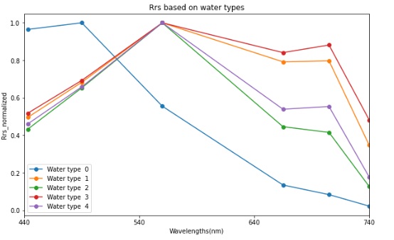

Fig. 1. Median of Normalised Rrs spectra, classified into five different water types with the k-means clustering technique, used for training the Chl-a estimation model.

Figure 2 presents scatter plots illustrating the model-derived Chl-a estimates for both the training and test datasets. Table 1 provides a summary of the model evaluation using seven error metrics: Bias, Intercept, Median Absolute Percentage Difference (MAPD), Normalised Root Mean Squared Error (NRMSE), Normalised Mean Absolute Error (NMAE), coefficient of determination (R²), and slope of the regression line.

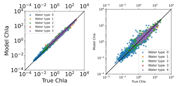Fig. 2. Scatter plot of model-derived Chl-a versus true Chl-a for train datasets (80%) [Left] and test datasets (20%) [Right].

Table 1. Performance evaluation of the present Chl-a estimation model against true values.

In conclusion, the Chl-a estimation ML model demonstrates satisfactory performance, with an R² value greater than 0.8 for test datasets. Furthermore, the MAPD of around 30% suggests that the model provides accurate estimates with minimal bias, making it a reliable tool for Chl-a prediction in the various optical water types.

​

Performance assessment of the Total Suspended Solids estimation model

Total Suspended Solids (TSS) (measured in g m^-3) is a key indicator of water quality, particularly in assessing the presence and abundance of suspended particles, primarily inorganic salts and sediments. Monitoring TSS helps in understanding the pollution level due to wastewater discharge or sediment transport.

Reflectance ratios at specific wavelengths are strongly correlated with turbidity, quantified as TSS concentration. In optically clear waters, the ratio of reflectance in the blue and green spectral regions is particularly sensitive to low concentrations of suspended particles. This sensitivity arises because suspended solids preferentially scatter and absorb light in the shorter wavelengths, causing measurable changes in the blue-to-green reflectance ratio. As TSS concentration increases, especially in more turbid waters, the spectral response tends to shift toward longer wavelengths, necessitating the use of red or near-infrared bands for more accurate quantification.

The present TSS estimation model, derived using machine learning (ML) techniques, was developed from approximately 14,600 paired observations of in-situ TSS concentrations and coincident remote sensing reflectance (Rrs) measurements, spanning five distinct optical water types across global inland and coastal waterbodies (Fig. 3). For model training and evaluation, 80% of the dataset was allocated to training (hereafter referred to as the train dataset), while the remaining 20% was withheld for independent validation (hereafter referred to as the test dataset).

Fig. 3. Median of Normalised Rrs spectra, classified into five different water types with the k-means clustering technique, used for training the TSS estimation model.

Figure 4 presents scatter plots illustrating the model-derived TSS estimates for both the training and test datasets. Table 2 provides a summary of the model evaluation using seven error metrics: Bias, Intercept, Median Absolute Percentage Difference (MAPD), Normalised Root Mean Squared Error (NRMSE), Normalised Mean Absolute Error (NMAE), coefficient of determination (R²), and slope of the regression line.

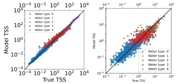Fig. 4. Scatter plot of model-derived TSS versus true TSS for train datasets (80%) [Left] and test datasets (20%) [Right].

Table 2. Performance evaluation of the present TSS estimation model against true values.

In conclusion, the TSS estimation ML model demonstrates satisfactory performance, with an R² value greater than 0.8 for test datasets. Furthermore, the MAPD of around 30% suggests that the model provides accurate estimates with minimal bias, making it a reliable tool for TSS prediction in the various optical water types.

​

Performance assessment of the a_CDOM(440) estimation model

Absorption coefficient of Colored Dissolved Organic Matter (a_CDOM) at 440 nm (measured in m^-1) is a key indicator of water quality, particularly in assessing the presence and abundance of decaying organic substances. It provides insights into the concentration of coloured dissolved organic matter, which influences water clarity, ecological health, and biogeochemical cycles.

Spectral reflectance ratios at specific wavelengths strongly correlate with the a_CDOM(440). a_CDOM(440) primarily influences light absorption in the ultraviolet and blue regions of the spectrum due to the presence of humic and fulvic substances derived from terrestrial and aquatic sources. In particular, the ratio of reflectance in the blue to green regions is sensitive to variations in a_CDOM(440), as CDOM strongly absorbs shorter wavelengths while exerting minimal influence on the green region. As a_CDOM(440) concentration increases, the absorption in the blue intensifies, leading to a decrease in reflectance in that region and thus altering the blue-to-green ratio. This spectral behaviour enables using blue-green reflectance ratios as effective indicators for estimating a_CDOM(440) across diverse aquatic environments.

The present a_CDOM(440) estimation model, derived using machine learning (ML) techniques, was developed from approximately 12,100 paired observations of in-situ a_CDOM(440) concentrations and coincident remote sensing reflectance (Rrs) measurements, spanning five distinct optical water types across global inland and coastal waterbodies (Fig. 5). For model training and evaluation, 80% of the dataset was allocated to training (hereafter referred to as the train dataset), while the remaining 20% was withheld for independent validation (hereafter referred to as the test dataset).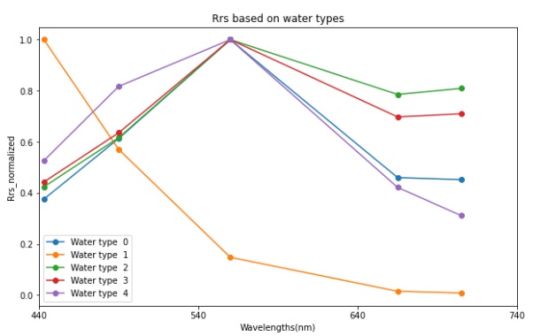

Fig. 5. Median of Normalised Rrs spectra, classified into five different water types with the k-means clustering technique, used for training the a_CDOM(440) estimation model.

Figure 6 presents scatter plots illustrating the model-derived a_CDOM(440) estimates for both the training and test datasets. Table 3 provides a summary of the model evaluation using seven error metrics: Bias, Intercept, Median Absolute Percentage Difference (MAPD), Normalised Root Mean Squared Error (NRMSE), Normalised Mean Absolute Error (NMAE), coefficient of determination (R²), and slope of the regression line.

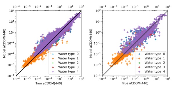Fig. 6. Scatter plot of model-derived a_CDOM(440) versus true a_CDOM(440) for train datasets (80%) [Left] and test datasets (20%) [Right].

Table 3. Performance evaluation of the present a_CDOM(440) estimation model against true values.

In conclusion, the a_CDOM(440) estimation ML model demonstrates satisfactory performance, with an R² value greater than 0.8 for test datasets. However, the MAPD calculated for the test dataset is marginally higher than the desired limit of 30% error. This increased error is mainly due to the absence of multiple green bands in the Sentinel-2 sensor, which restricts the model’s ability to accurately detect variations in CDOM absorption, especially in the green spectral region.